Why Is There a Gap Between Backtest and Live?

Every systematic strategy starts as a backtest.

This is the only proof we have before we allocate real money to the strategy. How much should we trust this number, and how close can we get to this when deployed live?

How big is the gap?

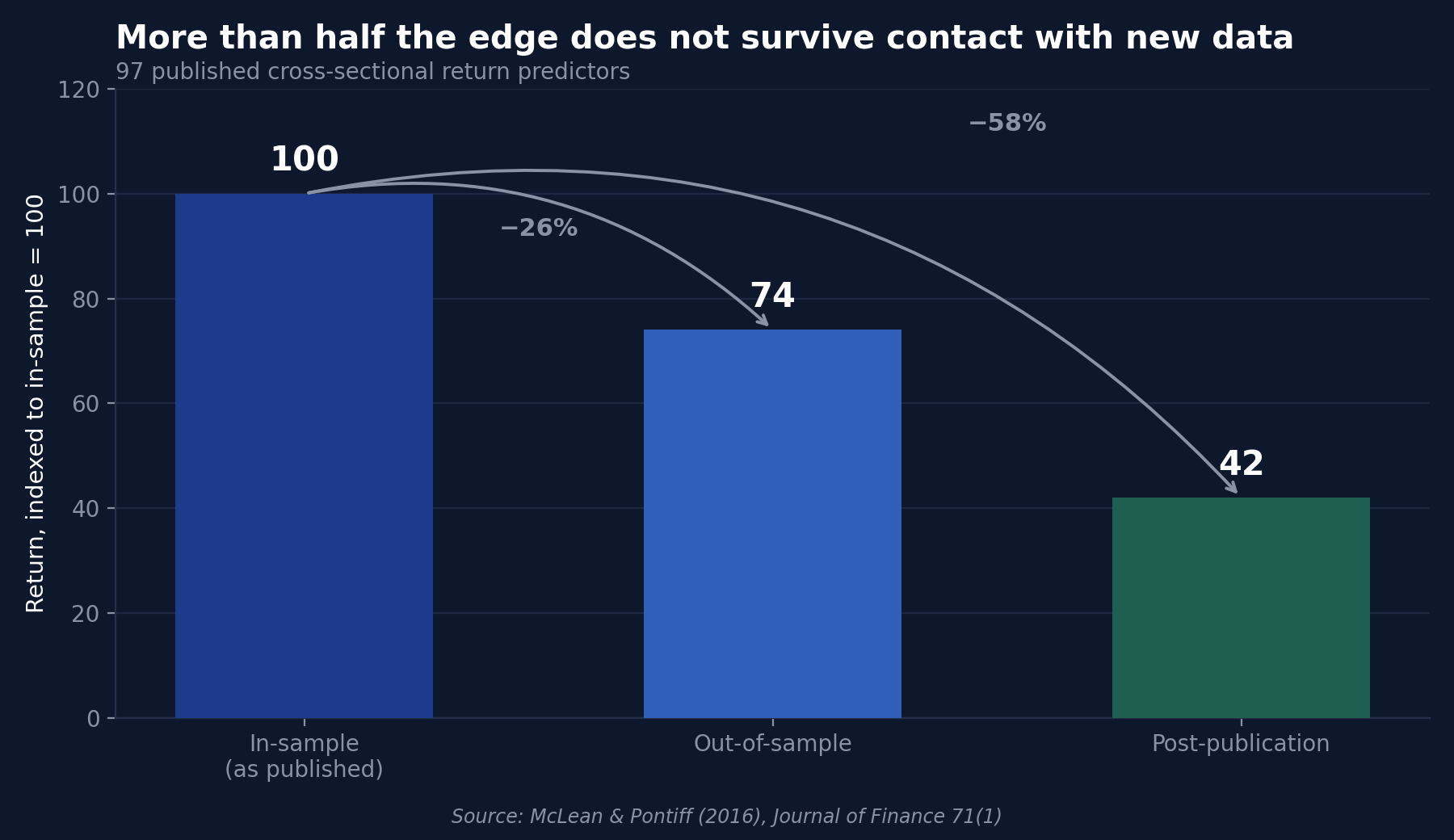
Edge vs. new data — McLean and Pontiff studied 97 published return predictors: returns were 26% lower out-of-sample, and 58% lower after publication, than originally claimed.

T-statistic threshold too low — Harvey, Liu and Zhu reviewed 316 published factors and argued the standard significance bar — a t-statistic of 2.0, a confidence level of 95% — is too low given how much has already been tested. Their proposed bar is 3.0, a confidence level of 99.7%. Their estimate: most published findings in financial economics are false.

Bar chart showing published return predictors falling from 100 (in-sample) to 74 (out-of-sample) to 42 (post-publication) — Fig. 1 — 97 published cross-sectional return predictors. Source: McLean & Pontiff (2016), Journal of Finance 71(1)

Are we overfitting?

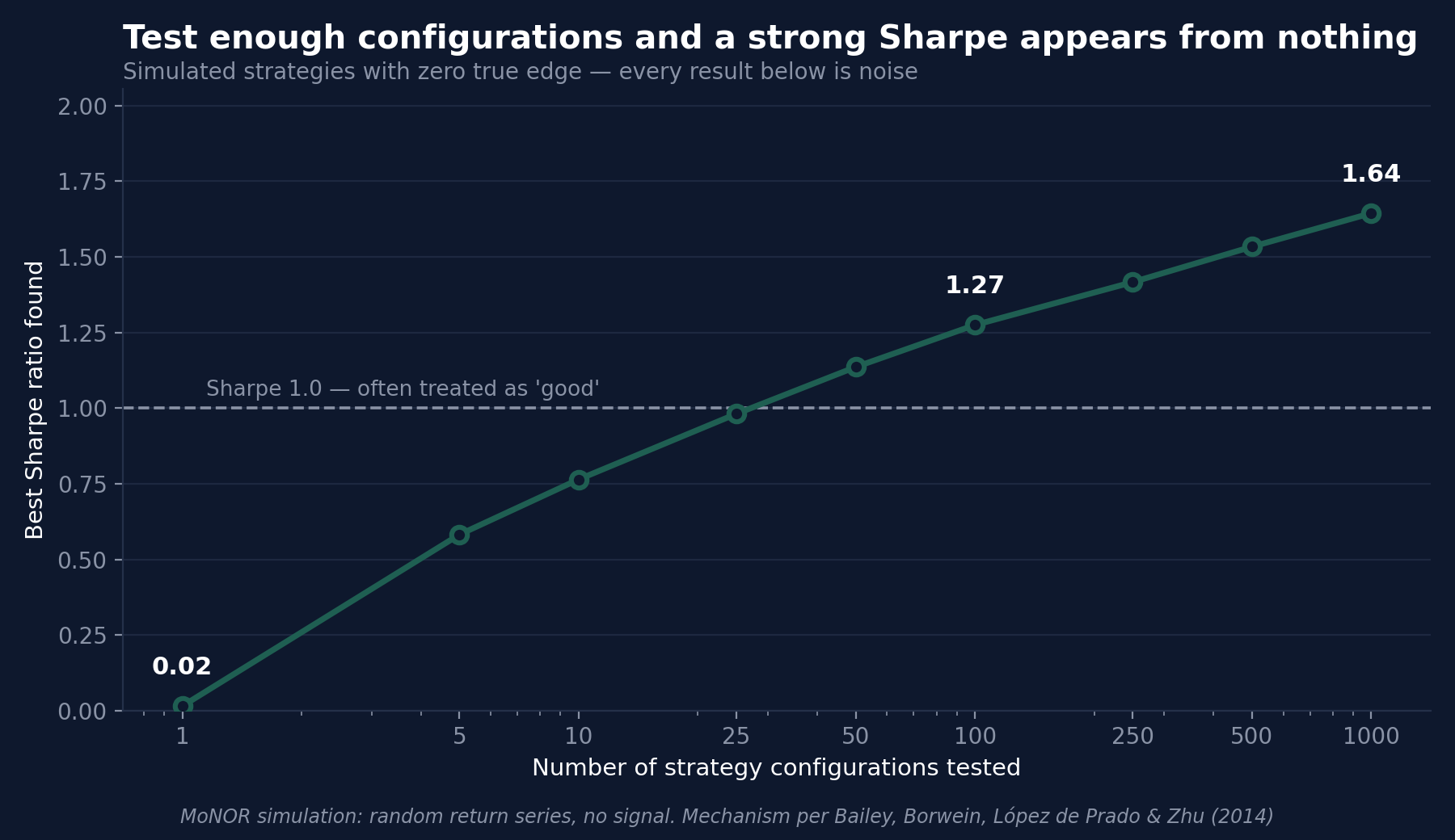
Bailey, Borwein, López de Prado and Zhu explain the mechanism — test enough configurations of a strategy and one looks great by pure chance. Almost nobody reports how many configurations they tried, so the overfitting stays invisible.

We tested this ourselves at MoNOR. We simulated pure random noise (should have zero edge). Then we picked the best of N configurations: with 1 trial, the best Sharpe found is near zero, correctly.

With 1,000 trials, the best Sharpe reaches 1.64 — a clear overfitting example.

Line chart showing the best Sharpe ratio found rising from 0.02 to 1.64 as the number of tested configurations increases from 1 to 1,000, despite zero true edge — Fig. 2 — MoNOR simulation: random return series, zero true edge. Every result shown is noise.

Three reasons the gap opens

Selection — a backtest is usually the survivor of many tested variations, most of which might not show a real edge.
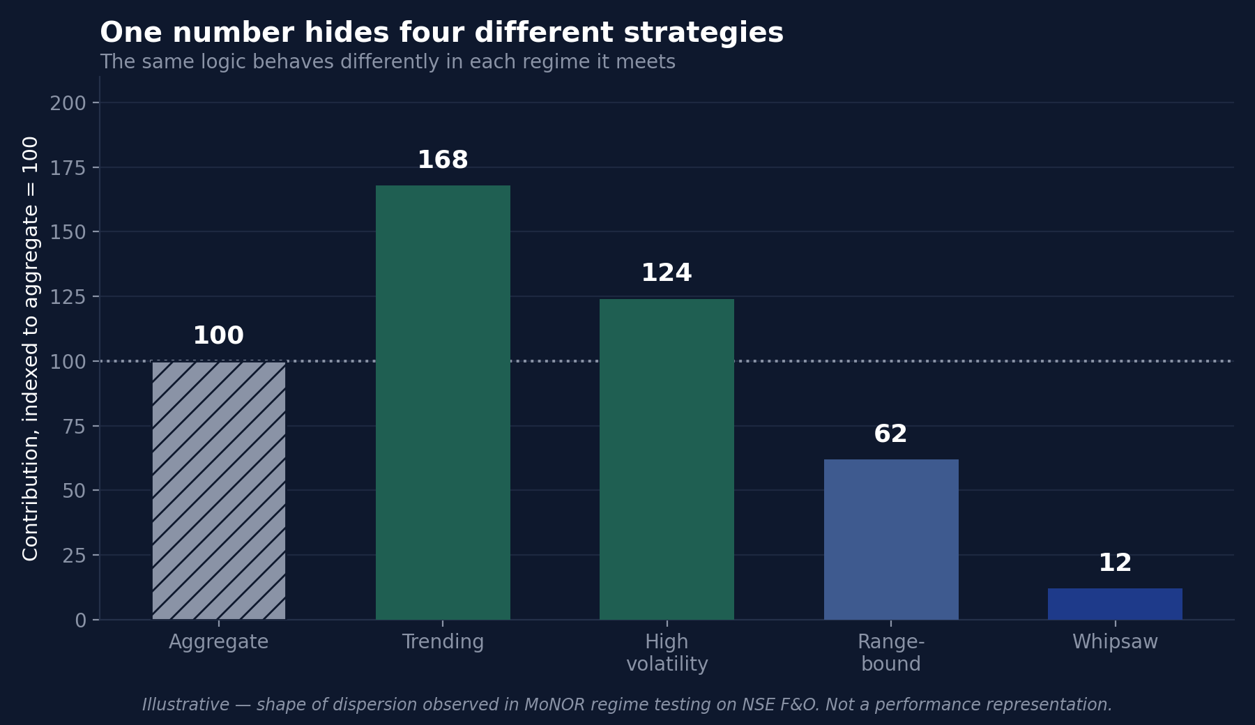
Regime dependence — the same strategy behaves differently across trending, ranging, high-vol and low-vol conditions. Our own NSE F&O testing found consistent drag in whipsaw and sideways regimes, invisible in the aggregate number.
Measurement error — in a multi-strategy stress test, one looked persistently weak. The weakness turned out to be a measurement artifact, not the strategy.

Bar chart showing contribution indexed to an aggregate of 100: trending 168, high volatility 124, range-bound 62, whipsaw 12 — Fig. 3 — Illustrative only, not MoNOR performance data. Shows how one aggregate number can conceal regime-level dispersion.

Closing the gap

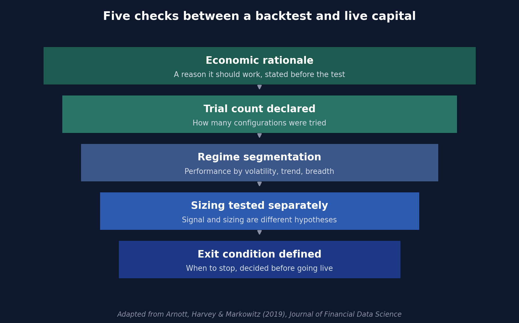
Arnott, Harvey and Markowitz proposed a research protocol for exactly this. Our 5-step version of it:

Rationale — start with a reason it should work, before testing it. A proper economic logic which should give you an edge.
Declare count — count and report every configuration tried. This number should be under a defined upper cap.
Regime segmentation — test by regime, not just in aggregate. Regimes may last longer than in backtest, which will hit hard on the backtest numbers.
Test sizing separately from signal — we found monthly sizing rules that were net negative against a flat baseline, invisible when bundled with the signal.
Continuous vigilance — the exit condition is defined before going live. Monthly review of performance parameters is needed to quickly identify an environment which isn't suitable for the given strategy, and when to stop.

Five-step funnel diagram: economic rationale, trial count declared, regime segmentation, sizing tested separately, exit condition defined — Fig. 4 — Adapted from Arnott, Harvey & Markowitz (2019), Journal of Financial Data Science.

Where we land

A backtest is a hypothesis. A positive result only gives you a go-ahead on the logic. A complete system for validating a strategy is critical before it is allocated capital — one that finds major weaknesses and decides whether the strategy is to be rejected or holds its ground. Most importantly, vigilance to spot when a strategy loses its edge, or sits in a regime where it is weak, is critical.

References

Bailey, D. H., Borwein, J. M., López de Prado, M., & Zhu, Q. J. (2014). Pseudo-Mathematics and Financial Charlatanism. Notices of the AMS, 61(5), 458–471.

Bailey, D. H., & López de Prado, M. (2014). The Deflated Sharpe Ratio. Journal of Portfolio Management, 40(5), 94–107.

Harvey, C. R., Liu, Y., & Zhu, H. (2016). ...and the Cross-Section of Expected Returns. Review of Financial Studies, 29(1), 5–68.

McLean, R. D., & Pontiff, J. (2016). Does Academic Research Destroy Stock Return Predictability? Journal of Finance, 71(1), 5–32.

Arnott, R., Harvey, C. R., & Markowitz, H. (2019). A Backtesting Protocol in the Era of Machine Learning. Journal of Financial Data Science, 1(1), 64–74.

Methodology note

T-statistic bar — in statistics, a t-statistic measures how many standard deviations an estimated effect is away from zero:

Traditionally, a t-statistic of ≥1.96 (roughly 2.0) corresponds to a 5% significance level (p<0.05).
If a researcher tests one single strategy and gets a t-statistic above 2.0, standard statistics says there is less than a 5% chance the result was just lucky noise.
A t-statistic of 3.0 corresponds to a 0.3% significance level (p<0.0027), a confidence level of 99.7%.

Fig. 2 is a Monte Carlo simulation, not sourced from a paper. For each N (1 to 1,000), we generated N independent daily return series (1,000 trading days, standard normal, zero true mean), computed the annualised Sharpe ratio for each, and recorded the maximum across the N series — averaged over several hundred repetitions per N. This mirrors picking the single best of N tested configurations. Every input is pure noise; this is not based on any MoNOR strategy.

Fig. 3 is illustrative only. The figures shown (168, 124, 62, 12, indexed to an aggregate of 100) demonstrate the shape of regime-driven dispersion referenced in the article. They are not MoNOR performance data.